top of page
Excel
WHAT IS A SPREADSHEET?
-
A spreadsheet referred to a worksheet is a file made of rows and columns.
-
That help sort data, arrange data easily and calculate numerical data.
-
Have the ability to calculate values using mathematical formulas and the data in cells.
-
There are many spreadsheet programs that can be used to create spreadsheet:
-
Google Sheets
-
iWork Numbers
-
Microsoft Excel
-
OpenOffice
-
and more
EXCEL INTRO
-
Microsoft Excel is a software program produced by Microsoft that allows users to organize, format and calculate data with formulas using a spreadsheet system.
-
This software is part of the Microsoft office suite and is compatible with other applications in the Office suite.
-
It Features the ability to perform basic calculations, use graphing tools, create pivot tables and create macros.
-
This is what a Excel application looks like, a collection of cells arranged into rows and colums to arganize and manipulate data.
-
They can also display data as charts, histograms, and line graphs.
-
Below is the Microsoft Excel spreadsheet looks like.

SHORT KEY
-
We can create keyboard shortcuts for any command with the Quick Access Toolbar.
-
Each button in the QAT has a keyboard shortcut assigned to it.
-
You will see numbers appear above the button.
-
Find & Replace. (Ctrl + H )

Alt
Press Alt to get Quick Access Toolbar.
-
Below is a listing of all the major shortcut keys usable in Microsoft Excell
-
Knowing keyboard shortcuts can speed up your work and save you time.
FORMULAE
-
A formula is an expression which calculates the value of a cell.
-
Functions are predefined formulas and are already available in Excel.
-
To enter a formula, execute the following steps.
-
1. Select a cell.
-
2. To let Excel know that you want to enter a formula, type an equal sign (=).
-
3. For example, type the formula A1+A2.
-
Sum:
-
The SUM function totals one or more numbers in a range of cells.
-
Select the blank cell in the row below the cells that you want to sum.
-
On formula bar, write =SUM(F8:F13)

-
Value function:
-
It converts a text string that represents a number to a number.
-
Syntax: VALUE (text).
-
See the below example to understand text format and number format difference.

This number is in text format.
('4333)
This number is converted into its numerical value.
=VALUE( D6 )
-
Text:
-
The Excel TEXT function returns a number in a specified number format, as text.
-
Format_text must appear in double quotation marks.

=TEXT (value, format_text)
The number to convert.
The number format to use.
-
Here an example of getting the text format to DAY from DATE and value to be in valid format.

Converting
Date Format to
Day Format
VLOOKUP & HLOOKUP
VLOOKUP: (Vertical Lookup)
-
VLOOKUP is an Excel function to lookup retrieves data from a specific column in the table.
-
It supports approximate and exact matching and wildcards for partial matches.
-
Lookup values must appear in the first column of the table, with lookup columns to the right.
-
Here is the example of adding a Mark value in another cell.

=VLOOKUP (lookup_alue, table_array, column_index, range_lookup)
-
Here is another example of VLOOKUP to find the semester of corresponding mark secured.
-
Start with an equal sign " = ".
-
Type =VLOOKUP ( E12, $D$2:$E$7,2,0) .
-
Click enter
-
It will change with respect to E12 value.
-
You can copy the formula.


To lock the selected array. (F4)
1 2
col_index_num
VLOOKUP with MATCH( ):
-
VLOOKUP and MATCH are the two formulas that are combined to perform this lookup.
-
You can change column index by MATCH( ) function inside the VLOOKUP() function.
-
A user can get the intersect value by changing ID(I4) and Column value(I5).
-
The difference is vertical lookup with Column lookup value.

Enter the ID
Enter Column Value
HLOOKUP: (Horizontal Lookup)
-
To retrieve data from a specific row in a table.
-
Lookup values appear in the first row of the table.
-
It is a built-in function in Excel that is categorized as a Lookup/Reference Function.

HLOOKUP( lookup_value, table, index_number, [approximate_match] )
Syntax:
-
Here is the example of how to use HLOOKUP function as a worksheet function in Microsoft Excel.

You can change the row value
Canstant Row value
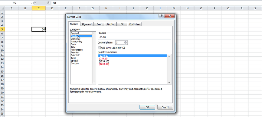
FORMAT CELLS
-
Here you can change the apperarance of a number without changing the number itself.
-
We can apply a number format ($,%, -, etc) or other formatting.
-
By default, Excel uses the General format for a number.
-
To apply a number format, use the 'Format Cells' dialog box.
-
To get the Format cells, right click on cell and click o Format Cells.

Ctrl
+
1
Activate Format cell
-
Here you can change the format you need.
-
There are different tabs allows you to change the font style, alignment, border etc.
-
To insert today's date, click a shortcut key as below.

Ctrl
+
;
To get Today's date.
Ctrl
+
3
To Convert date format.
Shift
+
FONT FILES (Download & Install)
-
Sometime when we are working in Microsoft Word, Excel, or other stuff, we want to add a new font.
-
Maybe some company has a different font that they use in their brochures and their brandings.
-
So here is an easy way to download and install a Font file that is not listed in MS office.
-
Below is the example, how to install Avenir font on the PC.
Step 1
-
The font Avenir is not installed on our PC as I can not find the font in Excel.

Avenir font is not installed
Step 2
-
Google your font name to download.

Step 3
-
Click on the Download button for further process.

Step 4
-
On the next procced page, click Download to download the file.
-
You can see the font file detail here.

Step 5
-
Open the downloaded Avenir-Free.zip file.

Step 6
-
Double click on files on after another to open and install.

Step 7
-
A window will pop-up asking for install.
-
Click the Install button to install the respective files.
-
The file will be installed on the PC.

Step 8
-
Re-open the MS office.
-
You can see the font is added to the list with a couple of versions.
-
Select the font to use.

You can use the installed Avenir font by clicking here.
bottom of page